Curriculum

Mathematics Grade XII

0/13

Text lesson

Chapter 13: Probability

Class 12 • Mathematics • Chapter 13

Probability

Updating chances with new information, from conditional probability through to Bayes’ theorem.

CBSE / NCERT Aligned

School Revise

Chapter Roadmap

Conditional Probability • Multiplication Theorem • Independent Events • Total Probability • Bayes’ Theorem • Random Variables and Mean

Reasoning with Uncertainty

Probability measures how likely an event is, on a scale from 0 to 1. The real power comes when new information arrives: once we know that one event has happened, the chances of related events shift. Conditional probability captures this updating, and it leads to some of the most useful results in all of mathematics.

This chapter builds from conditional probability to the multiplication theorem, independence, the total probability theorem and finally Bayes’ theorem, which reverses conditional reasoning and underlies medical testing, spam filters and machine learning. We finish with random variables and their mean, the expected value that summarises a whole distribution in one number.

Foundation

The conditional probability of A given B is P(A|B) = P(A ∩ B)/P(B), provided P(B) > 0. Two events are independent when P(A ∩ B) = P(A) P(B), so knowing one tells you nothing about the other.

Key Terms You Must Know

Term

Meaning

Example

Conditional probability

Chance of A given that B has occurred.

P(A|B) = P(A ∩ B)/P(B)

Independent events

Events where one does not affect the other.

P(A ∩ B) = P(A)P(B)

Total probability

Combining cases that partition the sample space.

sum of P(case) P(event|case)

Bayes’ theorem

Reversing a conditional probability.

find P(cause|effect)

Random variable

A number assigned to each outcome.

number of heads in two tosses

Mean (expectation)

The long-run average value of a random variable.

Σ x P(x)

Core Concepts, Step by Step

1. Conditional Probability

When we learn that event B has happened, the sample space shrinks to just B, and probabilities are recalculated within it. The conditional probability is P(A|B) = P(A ∩ B)/P(B). It answers the question: given B, how likely is A? This single idea is the foundation for everything that follows.

A two-stage probability tree: branch probabilities multiply along each path

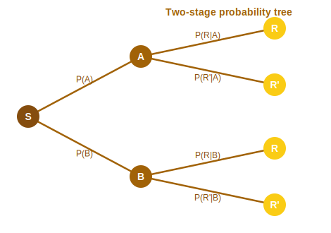
Probability tree from a start node splitting into events A and B, each leading to outcomes R and not R

2. The Multiplication Theorem

Rearranging the definition of conditional probability gives the multiplication theorem: P(A ∩ B) = P(A) P(B|A) = P(B) P(A|B). This lets us find the chance of two events both happening by multiplying along the branches of a probability tree, the standard way to handle multi-stage experiments.

3. Independent Events

Two events are independent when the occurrence of one leaves the probability of the other unchanged, that is P(A|B) = P(A). Equivalently, P(A ∩ B) = P(A) P(B). Independence must be checked, not assumed; many real events that seem unrelated are in fact dependent.

4. The Total Probability Theorem

Sometimes an event can happen through several mutually exclusive routes that together cover all possibilities, a partition. The total probability theorem adds the contributions: P(E) = Σ P(route) P(E|route). It is the natural tool when an outcome depends on which of several cases occurred first.

5. Bayes’ Theorem

Bayes’ theorem reverses the direction of conditioning. Given that an effect E occurred, it finds the probability it came from a particular cause: P(cause|E) = P(cause) P(E|cause) divided by the total probability P(E). It is the mathematics of updating belief in light of evidence, used everywhere from diagnostics to spam detection.

6. Random Variables and Their Mean

A random variable assigns a number to each outcome of an experiment, and its probability distribution lists each value with its probability. The mean or expected value, E(X) = Σ x P(x), is the long-run average. It condenses an entire distribution into a single representative number.

Key Results with Proofs

Result 1: The Multiplication Theorem

Statement. P(A ∩ B) = P(A) P(B|A).

Proof

The theorem is the definition of conditional probability, rearranged.

By definition P(B|A) = P(A ∩ B)/P(A), for P(A) > 0. – definition of conditional probability

Multiply both sides by P(A). – clear the denominator

P(A) P(B|A) = P(A ∩ B). – the result

By symmetry it also equals P(B) P(A|B). – second form

This is exactly the rule for multiplying probabilities along a tree branch.

Result 2: Independence Test

Statement. Events A and B are independent if and only if P(A ∩ B) = P(A) P(B).

Proof

Independence and the product rule each imply the other.

If A and B are independent then P(A|B) = P(A). – meaning of independence

Substitute into P(A ∩ B) = P(B) P(A|B): it becomes P(B) P(A). – substitute

So P(A ∩ B) = P(A) P(B). – forward direction

Reversing the steps shows the converse, completing the equivalence. – backward direction

Always verify the product equation rather than assuming independence.

Result 3: Bayes’ Theorem

Statement. P(Aᵢ|E) = P(Aᵢ) P(E|Aᵢ) / Σ P(Aⱼ) P(E|Aⱼ).

Proof

Bayes’ theorem is built from the multiplication and total probability theorems.

By the multiplication theorem, P(Aᵢ ∩ E) = P(Aᵢ) P(E|Aᵢ). – numerator

By total probability, P(E) = Σ P(Aⱼ) P(E|Aⱼ). – denominator

Then P(Aᵢ|E) = P(Aᵢ ∩ E)/P(E). – definition of conditional probability

Substituting the two expressions gives Bayes’ formula. – combine

It converts a forward probability P(E|cause) into the reverse P(cause|E).

Worked Examples

Example 1

Question: If P(A ∩ B) = 0.2 and P(B) = 0.5, find P(A|B).

▶ Show full working

Use the definition.

P(A|B) = P(A ∩ B)/P(B) = 0.2/0.5. – substitute

= 0.4. – divide

Answer: 0.4.

Example 2

Question: A fair die is rolled. Find the probability it shows a number greater than 4 given that it is even.

▶ Show full working

Condition on the even outcomes.

Even outcomes: {2, 4, 6}, so P(even) = 3/6. – sample space given B

Those greater than 4 and even: just {6}, so P(both) = 1/6. – intersection

P = (1/6)/(3/6) = 1/3. – conditional probability

Answer: 1/3.

Example 3

Question: Two cards are drawn without replacement from 52. Find P(both kings).

▶ Show full working

Multiply along the branches.

First king: 4/52. Given that, second king: 3/51. – two stages

Multiply: (4/52)(3/51) = 12/2652 = 1/221. – multiplication theorem

Answer: 1/221.

Example 4

Question: If P(A) = 0.6, P(B) = 0.5 and A, B are independent, find P(A ∩ B).

▶ Show full working

Use the product rule.

Independence gives P(A ∩ B) = P(A) P(B) = 0.6 × 0.5. – multiply

= 0.3. – result

Answer: 0.3.

Example 5

Question: Check whether tossing two fair coins gives independent events ‘first head’ and ‘second head’.

▶ Show full working

Compare P(A ∩ B) with P(A)P(B).

P(first head) = 1/2, P(second head) = 1/2, P(both) = 1/4. – probabilities

Since 1/4 = (1/2)(1/2), the events are independent. – check the product

Answer: Yes, they are independent.

Example 6

Question: Bag I has 3 red and 2 white; Bag II has 1 red and 4 white. A bag is chosen at random and a ball drawn. Find P(red).

▶ Show full working

Use the total probability theorem.

P(red) = P(I)P(red|I) + P(II)P(red|II). – total probability

= (1/2)(3/5) + (1/2)(1/5) = 3/10 + 1/10. – substitute

= 4/10 = 2/5. – add

Answer: 2/5.

Example 7

Question: In Example 6, given the ball drawn is red, find the probability it came from Bag I (Bayes).

▶ Show full working

Use Bayes’ theorem.

P(I|red) = P(I)P(red|I) / P(red) = (3/10)/(4/10). – Bayes formula

= 3/4. – simplify

Answer: 3/4.

Example 8

Question: A test is 90% accurate. A disease affects 1% of people. If someone tests positive, find P(disease) using Bayes (assume 90% true positive, 10% false positive).

▶ Show full working

Set up Bayes with the small base rate.

P(pos) = (0.01)(0.9) + (0.99)(0.1) = 0.009 + 0.099 = 0.108. – total probability

P(disease|pos) = 0.009/0.108. – Bayes

= 1/12 ≈ 0.083. – simplify

Answer: 1/12, about 0.083.

Example 9

Question: A coin is tossed twice. Let X be the number of heads. Write the probability distribution.

▶ Show full working

List values and probabilities.

X can be 0, 1 or 2. – values

P(0) = 1/4, P(1) = 2/4, P(2) = 1/4. – probabilities

Answer: P(0)=1/4, P(1)=1/2, P(2)=1/4.

Example 10

Question: Find the mean of X from Example 9.

▶ Show full working

Use E(X) = Σ x P(x).

E(X) = 0(1/4) + 1(1/2) + 2(1/4). – weighted sum

= 0 + 1/2 + 1/2 = 1. – add

Answer: E(X) = 1.

Example 11

Question: A die is rolled. Let X be the number shown. Find E(X).

▶ Show full working

Average of equally likely values.

E(X) = (1 + 2 + 3 + 4 + 5 + 6)/6. – each has probability 1/6

= 21/6 = 3.5. – compute

Answer: E(X) = 3.5.

Example 12

Question: If P(A) = 0.7, P(B) = 0.4 and P(A ∩ B) = 0.28, are A and B independent?

▶ Show full working

Compare with the product.

P(A) P(B) = 0.7 × 0.4 = 0.28. – product

Since P(A ∩ B) = 0.28 too, they are independent. – compare

Answer: Yes, independent.

Where You Meet This in Real Life

Medical testing

Bayes’ theorem converts a test’s accuracy into the real chance a positive result means disease, accounting for how rare the disease is.

Spam filtering

Email filters use Bayes’ theorem on word frequencies to estimate the probability a message is spam.

Weather forecasting

Forecasts update the chance of rain as new data arrives, a conditional-probability process.

Insurance

Premiums are set from expected values of claims, the mean of a payout random variable.

Quality control

Factories use conditional probability to decide how likely a batch is faulty given a sampled defect.

Practice Sets A–D

Practice Set A – Basics

A1. If P(A ∩ B) = 0.3 and P(B) = 0.6, find P(A|B).

▶ Reveal full working

Definition.

0.3/0.6 = 0.5.

Answer: 0.5.

A2. State the condition for A and B to be independent.

▶ Reveal full working

Product rule.

P(A ∩ B) = P(A)P(B).

Answer: P(A ∩ B) = P(A)P(B).

A3. Find P(A ∩ B) if P(A) = 0.5, P(B) = 0.4 and they are independent.

▶ Reveal full working

Multiply.

0.5 × 0.4 = 0.2.

Answer: 0.2.

A4. What does E(X) measure?

▶ Reveal full working

Expectation.

The long-run average value of X.

Answer: The mean / expected value.

Practice Set B – Conceptual

B1. Why does conditioning on B change probabilities?

▶ Reveal full working

Sample space shrinks.

Knowing B happened restricts attention to outcomes inside B.

Answer: Because the sample space shrinks to B.

B2. How is the multiplication theorem related to conditional probability?

▶ Reveal full working

Rearrangement.

It is the definition P(A|B) = P(A ∩ B)/P(B) rearranged.

Answer: It is the definition rearranged.

B3. What does Bayes’ theorem let you do?

▶ Reveal full working

Reverse conditioning.

Find the probability of a cause given an observed effect.

Answer: Reverse a conditional probability.

B4. When are two events independent?

▶ Reveal full working

Definition.

When the occurrence of one does not change the probability of the other.

Answer: When one does not affect the other’s probability.

Practice Set C – Application / Numerical

C1. A die is rolled. Find P(prime given odd).

▶ Reveal full working

Condition on odd.

Odd: {1,3,5}; primes among them: {3,5}. – outcomes

P = 2/3. – conditional

Answer: 2/3.

C2. Two cards drawn without replacement; find P(both aces).

▶ Reveal full working

Multiply branches.

(4/52)(3/51) = 12/2652 = 1/221.

Answer: 1/221.

C3. Bag has 4 red, 6 blue. Two drawn without replacement. Find P(both red).

▶ Reveal full working

Multiply.

(4/10)(3/9) = 12/90 = 2/15.

Answer: 2/15.

C4. X is the number of heads in two tosses. Find E(X).

▶ Reveal full working

Weighted sum.

0(1/4) + 1(1/2) + 2(1/4) = 1.

Answer: E(X) = 1.

Practice Set D – HOTS / Multi-step

D1. Bag I: 2 red, 3 black; Bag II: 4 red, 1 black. A bag is chosen at random and a red ball drawn. Find P(it came from Bag II).

▶ Reveal full working

Total probability then Bayes.

P(red) = (1/2)(2/5) + (1/2)(4/5) = 1/5 + 2/5 = 3/5. – total probability

P(II|red) = (2/5)/(3/5). – Bayes

= 2/3. – simplify

Answer: 2/3.

D2. A coin is biased with P(head) = 0.6. It is tossed twice. Find P(exactly one head).

▶ Reveal full working

Two disjoint orderings.

HT: 0.6 × 0.4 = 0.24; TH: 0.4 × 0.6 = 0.24. – two cases

Add: 0.24 + 0.24 = 0.48. – total

Answer: 0.48.

D3. A random variable X has P(1) = 0.2, P(2) = 0.5, P(3) = 0.3. Find E(X).

▶ Reveal full working

Weighted sum.

E(X) = 1(0.2) + 2(0.5) + 3(0.3) = 0.2 + 1.0 + 0.9. – compute

= 2.1. – add

Answer: E(X) = 2.1.

D4. A factory has machines A and B making 60% and 40% of items, with defect rates 2% and 5%. An item is defective. Find P(it came from machine B).

▶ Reveal full working

Total probability then Bayes.

P(defect) = (0.6)(0.02) + (0.4)(0.05) = 0.012 + 0.020 = 0.032. – total probability

P(B|defect) = 0.020/0.032. – Bayes

= 5/8 = 0.625. – simplify

Answer: 5/8, i.e. 0.625.

Chapter Summary

Everything in One Glance

Conditional Probability

P(A|B) = P(A ∩ B)/P(B); knowing B reshapes the chances.

Multiplication Theorem

P(A ∩ B) = P(A)P(B|A); multiply along tree branches.

Independence

P(A ∩ B) = P(A)P(B); one event does not affect the other.

Total Probability

P(E) = Σ P(case) P(E|case) over a partition.

Bayes’ Theorem

Reverses conditioning to find P(cause|effect).

Random Variable

E(X) = Σ x P(x) is the mean of the distribution.

Are You Exam-Ready?

8-Point Exam Quick-Check

If P(A ∩ B) = 0.24 and P(B) = 0.6, find P(A|B).

State the independence condition for A and B.

Find P(both heads) for two fair coins.

Write the formula for the total probability theorem.

What does Bayes’ theorem compute?

Find E(X) for a fair die.

Find P(A ∩ B) if P(A) = 0.3, P(B) = 0.5, independent.

Two cards drawn without replacement: P(both kings)?

School Revise Virtual Lab

Practice the concepts in this chapter with interactive simulations and visual tools.

Open the Virtual Lab →

Class 12 Mathematics Chapter 13: Probability, Complete Notes and Practice

These free Class 12 Maths Probability notes follow the NCERT 2026 to 27 syllabus and cover conditional probability, the multiplication theorem, independent events, the total probability theorem, Bayes’ theorem and random variables with their mean, with twelve worked examples and sixteen graded practice questions. Includes worked examples, step-by-step proofs and graded practice, free on SchoolRevise.com.